The CD Stack
How the pieces of the framework in the paper fit together, from the characteristic fields to the temporal closure.
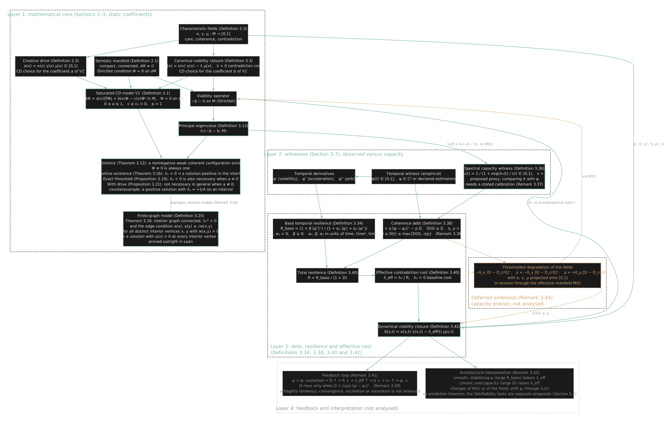
Reading the diagram
Layer 1: the mathematical core (Sections 2–3). The problem is posed on a semiotic manifold \(M\): compact, connected, with \(\partial M \neq \emptyset\) and the Dirichlet condition \(\Phi = 0\) on \(\partial M\) (Definition 2.1). The characteristic fields care \(\kappa\), coherence \(\gamma\) and contradiction \(\mu\) define the creative drive \(a = \kappa\gamma\mu\) (Definition 2.3) and, through the canonical closure (Definition 3.3), the viability potential \(b = \kappa\gamma - \lambda\mu\). These are the CD choices of the coefficients of the saturated model V1′ (Definition 3.1), the Dirichlet problem \(-\Delta\Phi = a|\nabla\Phi| + b\Phi - c\Phi^p\) in \(M\) with \(0 \le a \le 1\), \(c \ge c_0 > 0\) and \(p > 1\). The operator \(-\Delta - b\) has the principal eigenvalue \(\lambda_1\) (Definition 3.13). What is proved under these hypotheses: a nonnegative solution exists and the zero field is one (Theorem 3.12); \(\lambda_1 < 0\) gives a solution positive in the interior (Theorem 3.16); the condition is also necessary when \(a \equiv 0\) (Proposition 3.19); when \(a \not\equiv 0\) it is not necessary in general, since Proposition 3.21 gives a positive solution on an interval with \(\lambda_1 = +1/4\). The finite-graph model (Definition 3.25) is a separate problem (Remark 3.33): Theorem 3.26 gives a solution positive at every interior vertex when the interior graph is connected, \(\lambda_1^G < 0\), and the edge condition \(a(x), a(y) \le \sqrt{w(x,y)}\) holds on every edge between interior vertices; it is proved outright in Lean.
Layer 2: witnesses (Section 3.7). An empirical temporal witness \(\psi(t) \in [0,1]\) and its derivatives (volatility, acceleration, jerk) describe what a system is doing. The spectral capacity witness \(\psi_s(t) = 1/(1 + \exp(\lambda_1(t)/s))\) (Definition 3.36) maps the eigenvalue of the current operator into \((0,1)\), inside the range \([0,1]\) of \(\psi\). It is a proposed proxy; comparing it with \(\psi\) needs a stated calibration (Remark 3.37).
Layer 3: debt, resilience and effective cost (Definitions 3.34, 3.38, 3.40 and 3.42). The derivatives of \(\psi\) set the base resilience \(R_{\mathrm{base}}\) (Definition 3.34). Only operation above capacity, \(\psi > \psi_s\), feeds the coherence debt \(D\) (Definition 3.38), which decays at rate \(\rho\) and is bounded a priori by \(\max\{D(0), \eta/\rho\}\) (Remark 3.39). Debt lowers the total resilience \(R = R_{\mathrm{base}}/(1 + D)\) and raises the effective contradiction cost \(\lambda_{\mathrm{eff}} = \lambda_0/R\) (Definition 3.40). The effective cost and the fields at time \(t\) enter the dynamical closure \(b(x,t) = \kappa\gamma - \lambda_{\mathrm{eff}}(t)\mu\) (Definition 3.42). The closure supplies \(b(\cdot,t)\), so the operator and \(\lambda_1(t)\) are re-evaluated at each time.
Layer 4: feedback and interpretation (not analysed). The loop \(\psi > \psi_s \Rightarrow D\uparrow \Rightarrow R\downarrow \Rightarrow \lambda_{\mathrm{eff}}\uparrow \Rightarrow b\downarrow \Rightarrow \lambda_1\uparrow \Rightarrow \psi_s\downarrow\) is a fragility tendency (Remark 3.41). Debt rises only while \(D < (\eta/\rho)[\psi - \psi_s]^+\) (Remark 3.39), and the convergence, oscillation or saturation of the loop is not analysed. Under the architectural interpretation (Remark 3.43), smooth, stabilizing coherence lowers \(\lambda_{\mathrm{eff}}\), chronic overcapacity raises it, and changes of \(M(t)\) or of the fields shift \(\psi_s\) through \(\lambda_1(t)\). The falsifiability protocols are operational proposals, not derived from the PDE theorem (Section 5.2).
Deferred extension (Remark 3.44). Prolonged debt may erode the fields themselves, through thresholded laws for \(\kappa\), \(\gamma\) and \(\mu\) projected onto \([0,1]\), or erode the effective manifold \(M(t)\) and so act on the operator. Neither is analysed.
Status at a glance
| Layer | Status | Where |
|---|---|---|
| Mathematical core | Proved (Theorems 3.12, 3.16; Propositions 3.19, 3.21) | Sections 2–3, Figure 1 |
| Finite-graph model | Proved outright in Lean (Theorem 3.26) | Section 3.6, Figure 1 |
| Witnesses | Defined; \(\psi_s\) is a proposed proxy | Section 3.7, Figure 2 |
| Debt, resilience, closure | Defined, with an a priori bound; no well-posedness theorem for the coupled system | Section 3.7, Figure 2 |
| Feedback and interpretation | Interpretation; not analysed | Remarks 3.41 and 3.43, Figure 2 |
| Capacity erosion | Deferred | Remark 3.44, Figure 2 |